QuiXoT

QuiXoT
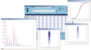Screenshot of QuiXoT, depicting different spectra and graphs used.
Last release: v.1.4.00
Release date: 20th Aug 2013
Download link: [[{{{link}}}]] Source code: QuiXoT at GitHub
Licence: Please read Licencing
Requirements
.NET Framework 2.0 or higher OS: Windows XP, Windows Vista or Windows 7

QuiXoT is an open source software created for the quantitation and statistical analysis of quantitative proteomics experiments. It has been developed at the Cardiovascular Proteomics Laboratory of Prof Jesús Vázquez, at the Centro Nacional de Investigaciones Cardiovasculares (CNIC), Madrid, Spain.

It has been developed in Visual C#, hence users must install the .NET Framework 2.0 or higher (not necessary for Windows 7 users), which can be downloaded from this link.

Download

You can download QuiXoT 1.4.00 from this link: File:QuiXoT 1.4.00.zip

Installation instructions

QuiXoT v1.4.00 is a portable, standalone application, so you do not need to install it to execute it.

Unzip the QuiXoT 1.4.00 folder (which you will find within the above-linked zip file) where you prefer in your computer. Then execute the QuiXoT.exe file (make sure it is the executable file, which has the QuiXoT logo, and not the QuiXoT.exe.config file, which will look as if it were called "QuiXoT.exe" when hiding file extensions). You may want to create a shortcut on your desktop or elsewhere to have fast access to QuiXoT.

Using QuiXoT

See also the article: DataGrid information in QuiXoT.

See also the article: Filtering data in QuiXoT.

See also the article: Sorting data in QuiXoT.

See also the article: Recommended parameters for QuiXoT strategies.

Part I: Checking an existent QuiXoT analysis

The QuiXML files

QuiXoT makes use of a QuiXML files, which is an ad hoc XML format created to manage the three levels of information treated: identification, quantitation and statistical information. To check a list of the different fields used in QuiXML files (i.e., the columns appearing in the main window of QuiXoT), you can check the article DataGrid information in QuiXoT.

After dragging and dropping the QuiXML file, you will have to choose the quantitation method.

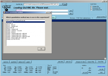
If you just want to see an existing QuiXoT analysis, you only need the corresponding QuiXML file. Just drag and drop that file on the main form, and select the quantitation method used, which will depend on the SIL method used (such as 18O, SILAC, etc) and the spectrometre used (sich as high or low resolution).

The binStack folder

The spectra are saved in a folder called binStack, which contains one or more .bfr files and one index.idx file. You do not need this folder if you just want to check the results of a QuiXoT analysis (such as the statistics, identifications or the quantitative information).

However, you will need it if you want to requantitate a spectrum, or see the spectrum itself (for example to compare the theoretical and experimental isotopic envelope, which are respectively in red and blue colours). If this is your case, then you should always have the QuiXML file and its corresponding binStack in the same folder (do not forget to move them together).

As far as the binStack and the QuiXML file are in the same place, you do not need to do anything else to load the spectral information.

The configuration files

In the location where you have copied your version of QuiXoT you will find a conf folder containing the configuration files. It contains three kinds of file:

• the QuantitationMethods.xml file, which contains the parameters of the different methods used. Here it is specified which labelling is associated to a method, or which is the spectrum type that contains the quantitative information (for instance, SILAC quantitation is performed in the full scan if a high resolution spectrometre has been used, but if it is a low resolution machine, then the quantitation is performed in the zoom scan immediately previous to the MS2 scan). Examples of other parametres that can be determined using this file are:

• width: the tolerance for the high resolution peaks
• deltaR: the mass difference between 16O and 18O
• sumSQtolerance_NG, the tolerance accepted for the sum of squares when comparing the theoretical and the experimental spectrum
• the iTRAQ masstags and their corrections

• several xml files which containg information such as the weights of each isotope, the composition of each amino acid or their posttranslational modifications. They also include the correspondence between the different residues and their symbols; for instance, "Y" means "tysorine", while "*" may refer to an oxidation in methionine, or a SILAC label on arginine. Examples of these files are:

• isotopes.xml
• aminoacids.xml
• aminoacids_SILAC.xml

• several xsd files, which are the XML schemas that contain the structure of the QuiXML file depending on each quantitation method. Some examples of these files are

• identifications_schema_18Ohighres.xsd
• identifications_schema_mascot_SILAC.xsd

Checking spectra by weight

Inspect quantifications with low Vs values. Sort the table by Vs (see Sorting data in QuiXoT) and inspect the spectra by using the spectrum button. At very low Vs values you will find completely useless spectra (bad fittings, mixtures, high background, etc). You can choose whether eliminating these spectra from the statistics by marking them with numLabel1 = 0, or filtering by a minimum Vs value (for instance Vs > 3). Non-quantifiable peptides (i.e. peptides not containing basic N-terminal residues in 18O-labeling or in SILAC) must also be excluded when calculating variances or performing the statistics.

Labelling efficiency for 18O labelling

If you have used 18O-labelling, you can check the labelling efficiency, prior to other analyses. Plot q_f versus Xs (consult how to create graphs). Since this plot does not differentiate between good and bad quantitations and hence plots together more and less accurate estimations of q_f, it is a good idea to eliminate bad quantitations from the plot by filtering out the data that do not have an arbitrary minimum Vs value (for instance Vs > 30 in ZoomScan-quantitated spectrum). Labelling efficiency must be above 0.8 for the vast majority of peptides. A cloud of points with q_f below 0.7 tending to curve towards the right (increasing Xs values) are indicative of a poorly-labeled experiment.

Part II: Analysing an experiment from scratch

Generating the files

Generate the QuiXML file containing the list of identified peptides. You can do this in different ways:

• if you have identified using SEQUEST (which includes Proteome Discoverer), you may use pRatio from either the .msf files (or the .srf files, if you use an older version of SEQUEST).
• if you have identified using Mascot, you may convert the .dat results file using MascotToQuiXML
• if you have used another program, you will need to convert your data into a tab separated text file, and then parse the resulting table using CSVToQuiXML

You will also need the binStack folder, containing the binary files with the spectral information. It can be generated in different ways:

• if you used Thermo RAW files, you can convert the spectra using RawToBinStack
• if you used Mascot generic files (mgf), you can convert the spectra using mgfToBinStack
• if your spectra are stored in a different file format, you should use an external converter to get a mgf file, and the use mgfToBinStack

Quantitating

A high resolution spectrum from an 18O-labelled experiment. Notice the light species (the four peaks at the left) and the heavy species (the peaks 5th to 8th). The theoretical peaks are red colour, while the original, experimental spectrum is blue colour. You can see a contaminant (or perhaps another less abundant peptide) on the right side of the spectrum (of course, only blue colour, as it does not match a theoretical spectrum in this case).

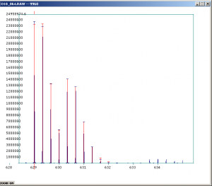
To quantitate a single spectrum just select a row by clicking on its left side, and the press the quantitation button. You will see that several columns that were empty (such as q_A or q_log2Ratio) are now filled. Additionally, if you are visualising the spectrum, you will see that a red colour spectrum has appeared, superposed to the blue colour experimental spectrum. Both spectra may match better or worse depending on the spectrometre performance, level of noise, artefacts, and the fact that the identification might be correct or not. The more similar the theoretical and the experimental spectra are, the higher the assigned weight will be (which you will find in column Vs). On the other hand, if the spectrum is very bad (for example because it contains several contaminants that are mixing with the signal from the peptide), then it will be assigned a low weight, which means it will have a very low impact in the posterior statistics compared to other spectra.

To quantify the whole experiment, simply select all the rows (by clicking on the top-left corner of the datagrid) and press the quantitate button. Take into account that this might take between a few seconds to several hours depending on the amount of spectra and the quantitation method used.

Performing the first statistics

Introduce an initial set of statical parameters (k and variances) for the null-hypothesis model by using the change_values link. You can find a list of typical values for these parameters. Make an initial estimation of variances by pressing the var calc button. At this step you will have to tell QuiXoT which columns are going to be used as Xs and Vs (this is useful for multichannel labelling approaches such as, for instance, iTRAQ data, which contains several Xs and Vs values depending on the labels that are to be compared). Accept the newly calculated variances and perform the statistical analysis by pressing the stats button.

Inspecting spectra and peptides

Graph window showing the Ws vs Xs-Xp plot (i.e., the weight of each scan in the Y-axis, compared to the log2ratio of each scan centred on its peptide). In this particular case, no outliers appear in the graph.

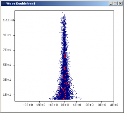
Inspect the presence of outliers at the scan and peptide levels by using the graphs button and setting Ws (or Wp) as X, vs Xs (or Xp) as Y, to check whether these data are influencing variance calculation. Sort out the data (see Sorting data in QuiXoT) by FDRs (or FDRp) and check the rows having low FDR values (below 0.05 they are statistically considered as outliers). Typically a negligible proportion of outliers may be found (less than 1% of total); this is normal. However, if the number of outliers is too high, it may be indicative of quantification artefacts and/or problems in the labelling protocol.

Common artefacts at the scan level are rare and may be produced by

a) problems in mass calibration (spectra cannot be fitted to the theoretical mass envelope)

b) excesive noise and/or fluctuations in the detector

c) inadequate fitting parameters in the configuration files.

Common artefacts at the peptide level are, however, much more frequent when peptides are post-digestion labelled (which does not include SILAC). They include:

a) incomplete digestion of one of the samples (this may be easily checked by selecting peptide subpopulations using the st_PartialDig field and the filter tool in Vs versus Xp plots)

b) non homogeneous methionine oxidation in the samples to be compared (this may be easily checked by filtering out by the st_Meth field)

c) partially labelled peptides (with 18O-labelling this is indicated by q_f)

If any of these artefacts are encountered, outliers should be eliminated from variance calculation or statistics by using the filter tool.

A further inspection of proteins showing significant expression changes (low FDRq values) is recommendable at this step, since keratins and other external contaminants like trypsin may not be well-balanced in the two samples and introduce an artefactual variance at the protein level. Eliminate all the quantifications related to these contaminants from the statistics by applying an appropriate filter (consult Filtering data in QuiXoT).

Variance calculation

A Zq plot, showing the experimental curve (blue) vs the theoretical N(0,1) distribution (red); click on the image to enlarge.

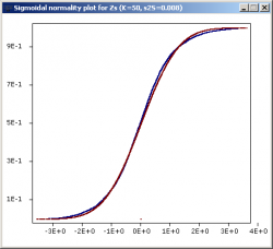
Recalculate variances (var calc button), accept the resulting values and repeat the statistics (stats button). Check the null hypothesis behind the data. Press the graphs button, and select either Zs, Zp or Zq as X values and the sigmoidal normality plot option to check the null distributions at the scan, peptide or protein level, respectively. If everything is fine and the k constant and variances are properly calculated, these data (blue line) should produce a sigmoid corresponding to the normal distribution around an average of zero with a standard deviation of one (red line). Deviations of the blue curve in relation to the red curve indicate that the null hypothesis is not valid to analyse the data. There are different kind of deviations:

• if the blue curve is less steep (less accused slope) than the red curve, it means that the variance has been underestimated.
• If the blue curve is steeper (higher slope) than the red curve, then the variance has been overestimated.
• if the blue curve agrees with the red curve in the middle but is higher at low values and/or lower at high values, it may be indicative of the presence of outliers.

Although the variances can be adjusted manually (using the change_values link) until experimental and theoretical curves agree, it should be noted that these deviations are usually indicative of the presence of contaminants, artefacts or outliers that disturb normality and make variance estimation inaccurate. Therefore, it is recommendable to inspect the underlying problem before manual adjustment of variances.

Using the linear normality plot

A more sensitive method to detect deviations from normality is to use the linear normality plot. In this graph a normal distribution produces a straight line, and the points outside the line correspond to outliers.

A note of caution: estimation of variances from an experiment can only be done when the number of expression changes (or outliers) is low enough not to disturb the underlying normality distribution. As the proportion of proteins having expression changes increases, a point may be reached where there is no way to establish what is the true variance of the null hypothesis (i.e. the underlying experimental variance of the non-changing proteins). In such cases the only solution is to make a parallel, null-hypothesis experiment to estimate the true protein variance and use this variance to analyse the results from the real experiment. This is a classic problem in statics and has nothing to do with QuiXoT performance.

Final statistics

Once the null hypothesis at the three levels (scan, peptide and protein) is correctly established (i.e. normality is met and variances are correctly calculated), then the final statistical analysis may be performed by pressing the stats button. Protein expression changes are usually considered as significant when FDRq is lower than 0.05 (meaning that 5% of significantly changing proteins show expression changes by chance alone). It is easy to highlight the changing proteins in a Wq vs Xq plot by applying the filter tool to the FDRq field. Note that FDRq < 0.05 is a multiple-hypothesis criterion and is a much more stringent condition than abs(Zq) > 1.96, which corresponds to a 0.05 probability that the protein, considered alone, deviates from the normal distribution.

References

• A. Ramos-Fernández, D. López-Ferrer, and J. Vázquez, «Improved method for differential expression Proteomics using trypsin-catalyzed 18O labeling with a correction for labeling efficiency», Mol Cell Proteomics 6, 1274-1286 (2007) (DOI: 10.1074/mcp.T600029-MCP200)

• S. Martínez Bartolomé, F. Martín-Maroto, P. Navarro, D. López-Ferrer, M. Villar, A. Ramos-Fernández, J.P. García-Ruiz, and J Vázquez, «Properties of average score distributions of SEQUEST: the probability ratio method», Mol Cell Proteomics 7, 1135-1145 (2008) (DOI: 10.1074/mcp.M700239-MCP200)

• I. Jorge, P. Navarro, P. Martinez-Acedo, et al., «Statistical model to analyze quantitative proteomics data obtained by 18O/16O labeling and linear ion trap mass spectrometry: Application to the study of VEGF-induced angiogenesis in endothelial cells», Mol Cell Proteomics , (2009) (DOI: 10.1074/mcp.M800260-MCP200)

• P. Navarro and J. Vázquez, «An improved method to calculate False Discovery Rates for peptide identification using decoy databases», J. Proteome Res. 8, 1792–1796 (2009) (DOI: 10.1021/pr800362h)