Exploring QuiXoT features

.Here we describe some of the features of QuiXoT you can use in everyday's work analysing quantitative proteomics experiments. If this is the first time you run the program, you might be interested first in checking the unit tests for QuiXoT.

Analysis 1

We will check some features using the 18O experiment using high resolution spectrometry, which we can see in the Test 1 of the unit test. If you didn't generate the QuiXML file (including quantification and statistics) following those steps, you can use the file VSMC_QuiXML_bs_quant_stats.xml in the VSMC_result folder (remember to move this file together with the binStack if you want to see the spectra; or just use the QuiXML alone if you do not need them).

1.1 Getting started

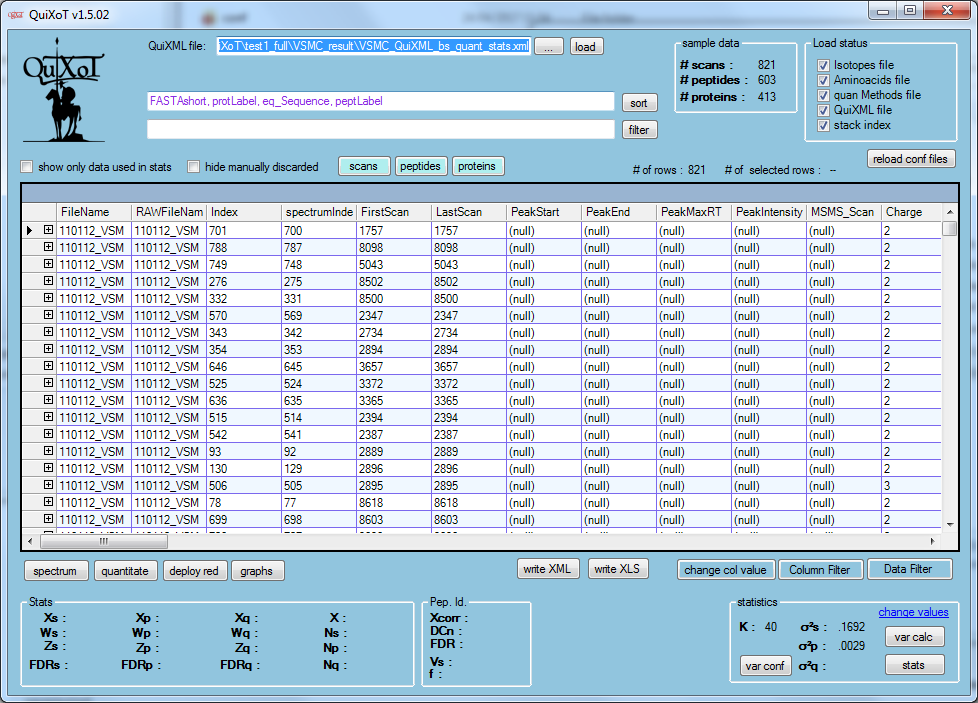
Open QuiXoT.exe, drag and drop anywhere on its window the abovementioned QuiXML file, and select the 18, HR, SEQUEST strategy. You should see this window:

1.2 Managing spectra

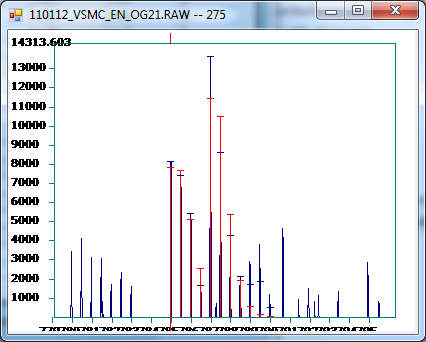
We might want to start checking how are the spectra (if you did not copy the binStack, you can skip this and go to generating graphs). Click on button spectrum, and then click on any row in the datagrid. For the fourth row (with FirstScan = 8502) you should see something like this

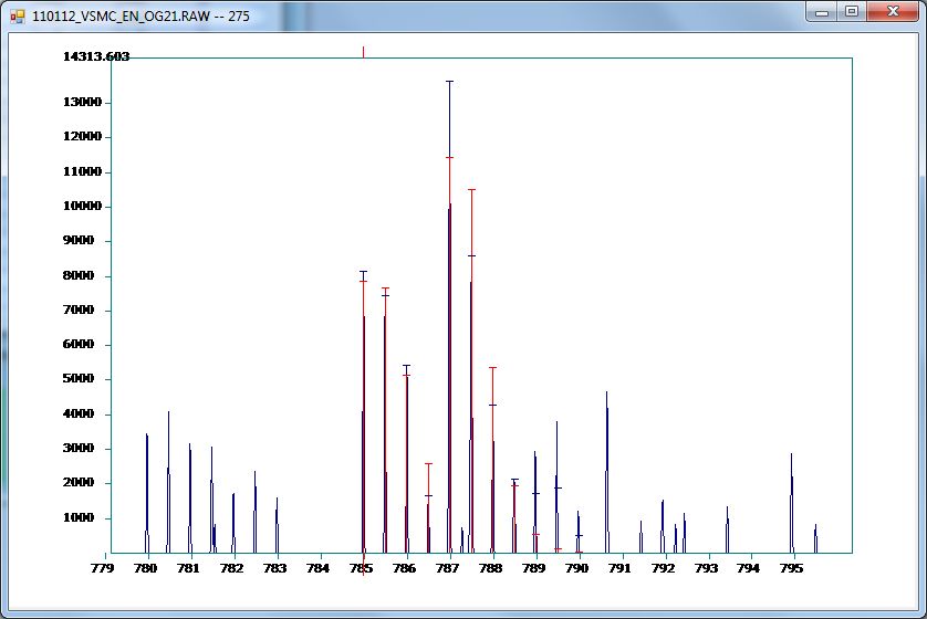
The experimental spectrum is drawn blue colour, while the red colour is the theoretical prediction (taking into account the peptide sequence, the isotope distribution, the labelling, and the labelling efficiency). The "lids" of the quantified peaks depict the tolerance used to consider if the theoretical peak matched (or not) the experimental one (note that there is a minimum "lid size" to visualise it). We can enlarge it to see better:

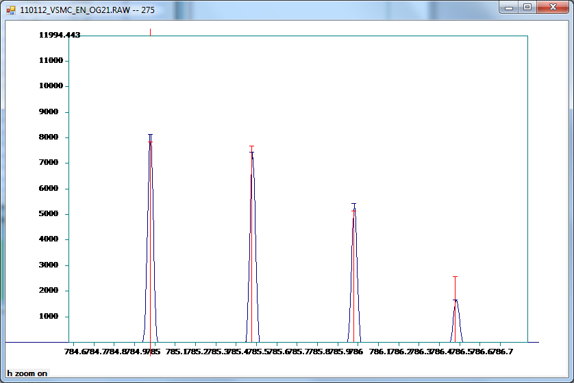
Or select the first four quantified peaks with the mouse (click and drag horizontally):

In this view we can see that apparently no co-eluted peaks are present.

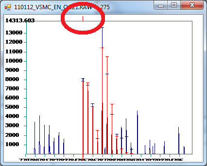
Note that on the top of the screen we have an indicator of which is the precursor mass of the peptide that has been matched:

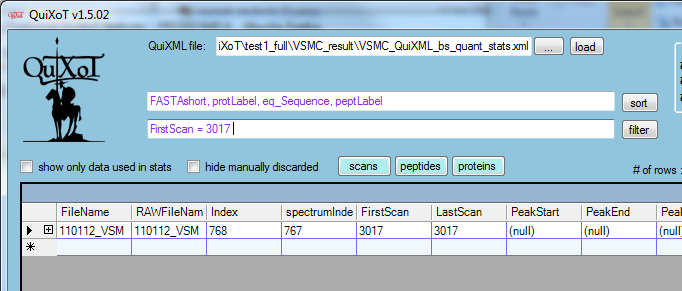
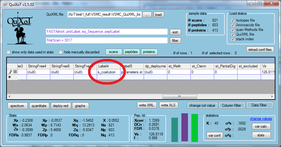
Let's look at a specific spectrum. To make it faster, we will filter the spectrum with FirstScan = 3017 (write the filter in the filter field and then click on the filter button:

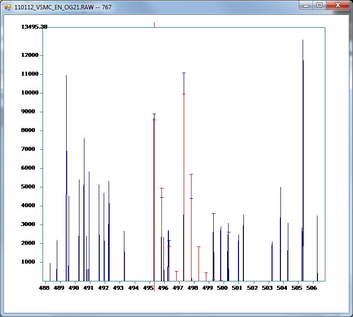
The open the spectrum, enlarge

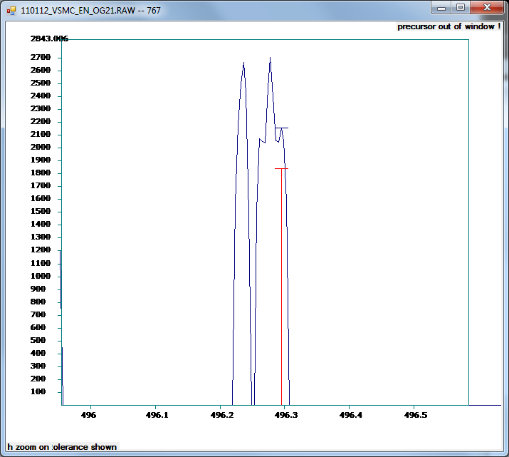
And then select the third quantified (red) peak:

(Note the warning on the top: the precursor is outside this window.)

This is a clear example of a co-eluted peak, so we can label that peak to filter it out of the statistics later. We can go to the Label4 column, and directly write down s_coelution (or any other tag we prefer, as far as we can filter it easily later; starting the tags related to scans as s_, those related to peptides as p_, and those related to proteins as q_ is a good practice to distinguish between filters):

We can right-click on the spectrum to either zoom out or export data to a text file that can be treated by another software.

1.3 Generating graphs

Close the spectrum-window, and remove the filter in the filter field (delete and click on filter button).

You can see that in the lower left corner there is a lot of information about every quantification. You can go down with the mouse and this information will show the information of each scan-peptide-protein of every row:

The details of this are explained in DataGrid information in QuiXoT.